“Measure what can be measured, and make measurable what cannot be measured.”

– Galileo Galilei

After (suffering) experiencing IGCSE for 1.5 years, I have to say, I’m not amused with the workload I’ve had to deal with, although I know it’ll only get worse from here. Still, I have to say I’m insanely grateful for all that I’ve had the opportunity to learn and understand, and I’m even more grateful that I’ll have the chance to continue my education with IB program (and hopefully do well enough with that).

Before I can lounge and relax, however, now that the semester assignment is coming to an end, I have to, of course, write up a math e-journal to get 30% of my final grade. For this particular assignment, we’ll be discussing IB questions that should hep us gain a better understanding about math.

Part a: Investigation A: A Very Safe Plane

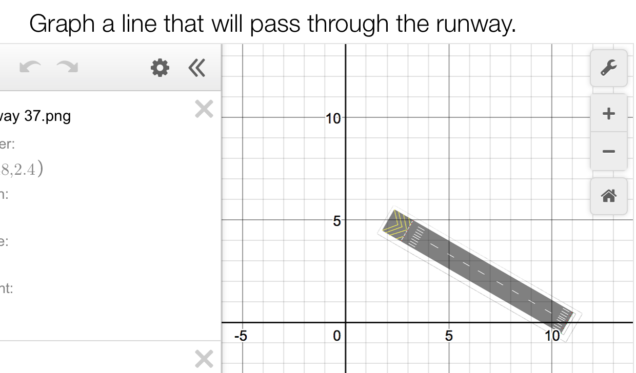
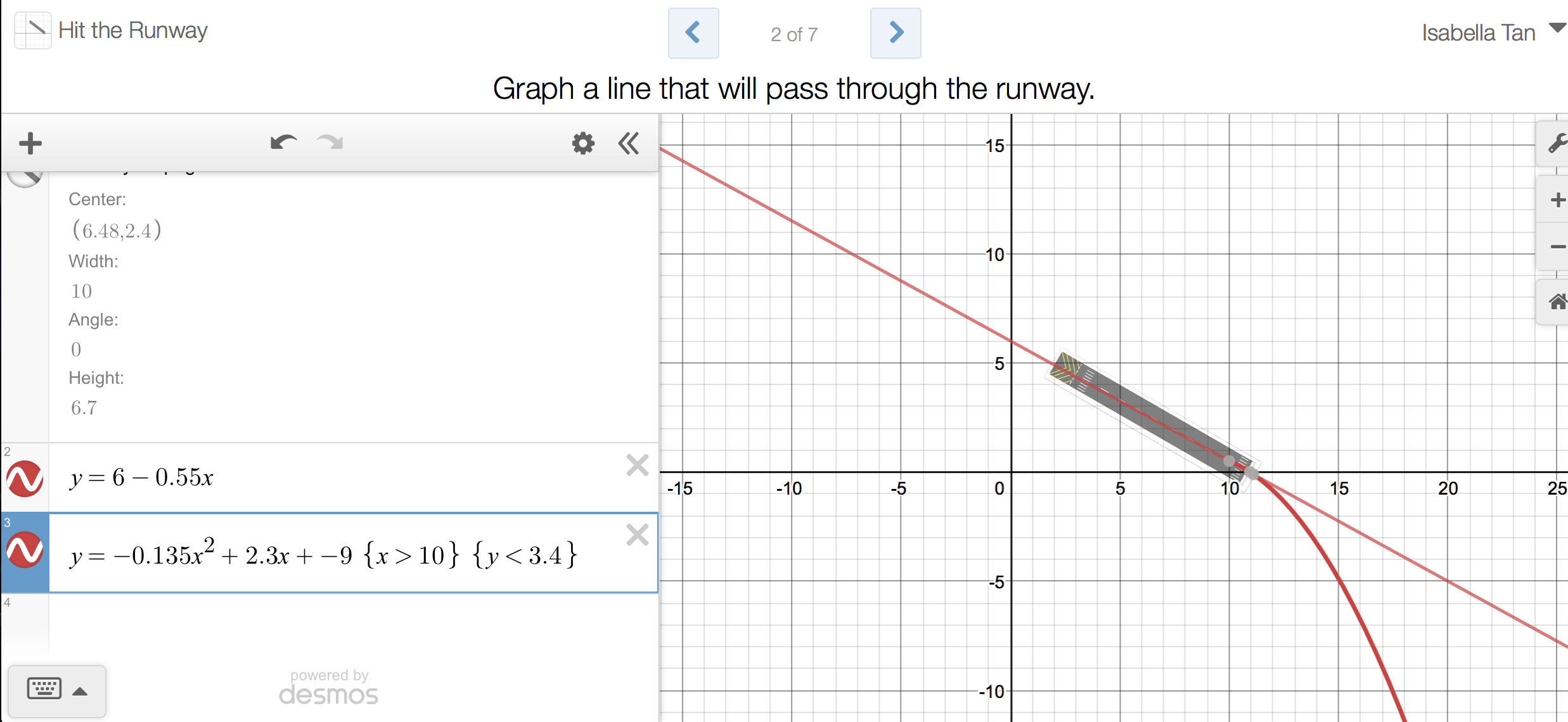
You’re sitting in the cockpit, leaning relaxedly but just straight enough that if needed, you could quickly commandeer your plane manually. Behind the relatively narrow, aluminium door behind you sits rows upon rows of people awaiting that small thump that will tell them they’ve arrived. After a long 8 hours, it’s finally time to land. Will you make it through the runway?

We were given 7 runways and for each of them, we were supposed to construct a line which would represent a plane’s path as it descended onto an airport’s runway. The main goal was, of course, to ensure our flight’s mortality rate was 0%.

The topics involved in this task are, of course, geometry, particularly linear equations, or equations where the highest power is 1.

Of course, we all know that the formula for a straight line is y=mx+c where m is the gradient and c is the y-intercept, or where the line cuts y-axis. To solve these questions, this one in particular:

I first entered the variable y and the ‘=’ sign, before inputting the y-intercept; where I predicted the line would cut the y-axis by imagining a line passing through the white stripes symbolizing the middle of the runway that would extend to the y-axis. In my mind, this line cut the y-axis at 6, so the equation became y=6. Of course, this would produce a completely horizontal line if I left it as is, so I turned to find the gradient of the line.

Now that I had one of the coordinates of the line – (0, 6) from the y-intercept – I turned to find the point where the line cut the x-axis. Once again, I extended my line and found that it would cut the x-axis at the point (11, 0).

With these two points, I could find the m or gradient of the line using the formula (y2-y1)/(x2-x1). This got me to (0-6)/(11-0), which is -6/11, which rounds off to -0.55.

Therefore, the line equation I entered for that question was y=6-0.55x.

While I used a line and line equation to solve this problem, as advised by some JC students, it’s also possible for the plane to curve or circle the runway before touching it instead because, in real life, sometimes the plane isn’t parallel with the runway and needs to turn to reach it. For this investigation, I added a curve showing what a plane might turn like to get to the run away. This was done by playing around with dismiss and changing the numbers for variables a, b and c of the quadratic equation and adding limits for the curve so that the plane didn’t overshoot the runway.

Part B: Investigation B: Koch‘s Irritable Snowflakes

Iteration no.	Perimeter (cm)	Area (cm^2)
1	243	2841
2	324	3788
3	432	4209
4	576	4396

Overall, the model for the area and perimeter would be:

Perimeter = 81/3^(iteration no-1) x 3(4^(iteration no-1))

Area = (previous iteration’s area)/3^(iteration no) x 3(4^(iteration no-1))

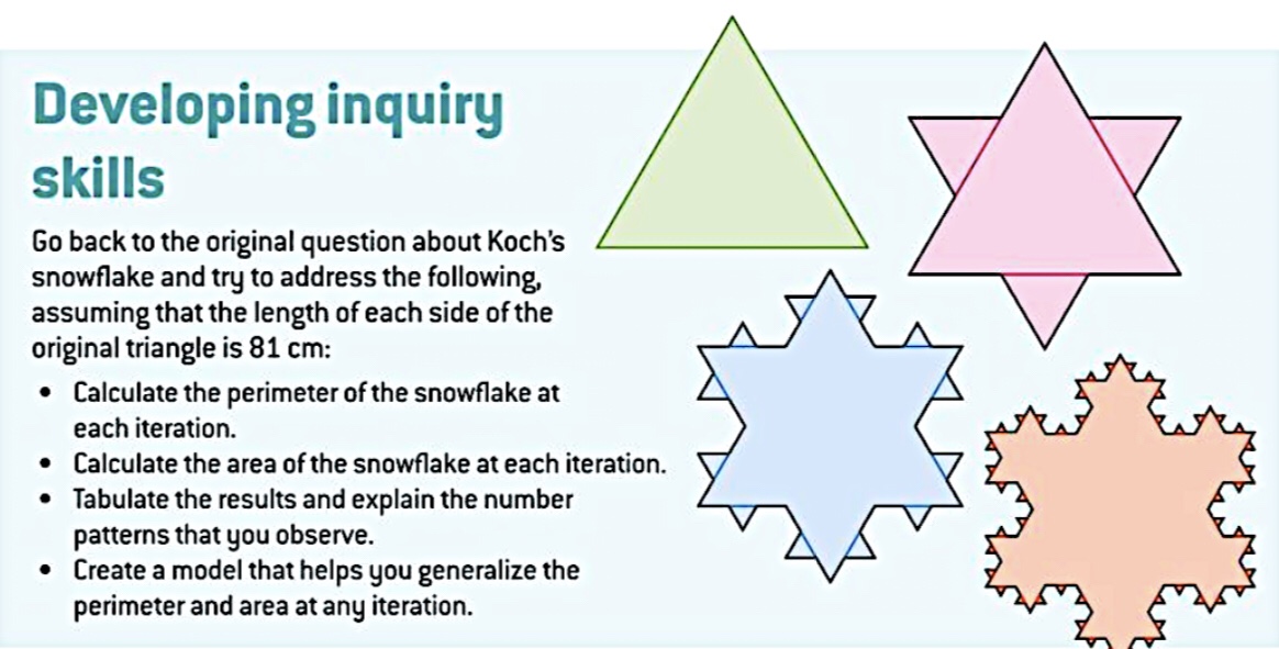
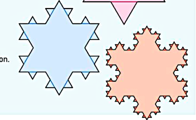
So, this time for this task, we need to explore koch’s triangle and find the perimeter and area for its different iterations, tabulate the results and find a formula we can use to find the perimeter and area of any iteration of Koch’s triangle. The topics involved here are the area and perimeter formulas of a triangle, geometry, geometric sequences and infinity.

Anyway, the key to solving the perimeter and area of his snowflakes is to know the length of the triangles, as all his triangles are equilateral and every other variable we need to know can be calculated using this length.

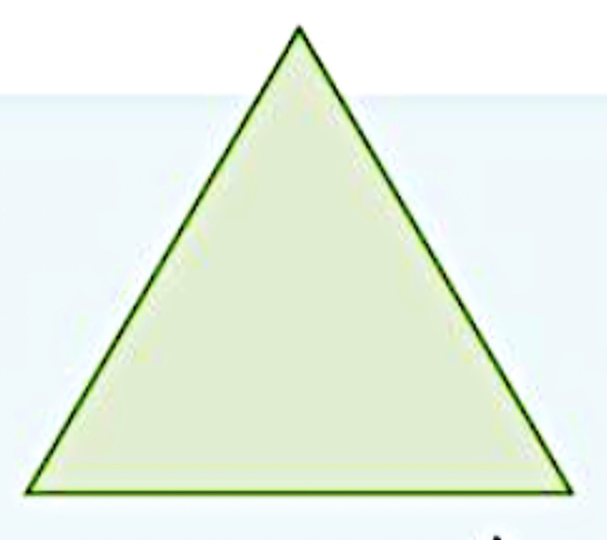
We initially know the length of the largest triangle is 81 cm.

Next, we can divide this large triangle into smaller triangles by dividing it into the protruding smaller triangles added in the first iteration of the snowflake.

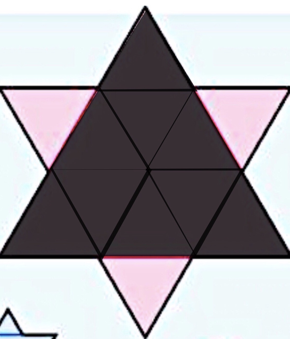
As we can imagine, one side of the original triangle, makes up three smaller triangles’ lengths. And as all the triangles are congruent and equilateral, we can deduce that the length of the smaller triangle is 81/3, which is 27 cm.

This goes on for the next two iterations of the triangles; we just keep dividing the previous iterations’ length by 3. As a result, we can make a formula for the length of each side of the triangles’ iteration:

Length (iteration no) = 81 /3^(iteration no-1)

Therefore, to find the perimeter of each triangle, we just need to multiply the length of the triangle we found using the above formula and multiply it by the number of sides a triangle has.

As for the area of the iterations, for the first triangle, obviously, we can use the standard triangle formula, which is 1/2 x base x height, which in this case becomes 1/2 x 81 x height. Since it’s an equilateral triangle, the way we can find the height is to cut the triangle in half to make two right angle triangles and use Pythagoras’ theorem. This would make the height 70.15 round off to two decimal places. Therefore, the area of the first triangle would be 2841 when round off to whole number.

The next few iterations are more troublesome. For the next triangle, we can just divide the previous iteration’s area by 9 to get the area of the smaller triangles, which is 315.68, and then multiply it by the number of smaller triangles in this iteration, which is 12 as the original triangle had 9 smaller triangles and 3 additional smaller triangles were added with one on each side of the original triangle. So the second iteration’s area would be rounded off to 3788.

For the next iteration, we divide the area of the smaller triangle by 9 again to get the are of the smallest triangle in this iteration, multiply this by 12 then add it to the area of the pervious triangle. This goes on for the next iteration.

From the table at the very gaining of the part, we can see that the perimeter for the iterations of Kochs’ triangles make a up a geometric sequence whose formula is Un = 729/4 x 4^(iteration no)/3. The increments between these numbers are always some multiple of 3. This shows that the perimeter of Koch’s snowflake is a geometric sequence.

The area of the iterations, on the other hand, are increasing but its increments are decreasing from 947 to 421 to 187. The area is not a series.

As Koch’s fractal snowflake can infinitely add more triangles to itself as it will always have a straight line that can have a triangle added to it every iteration, the perimeter of Koch’s triangle is considered boundless and, therefore, infinite.

If you’d like to further explore and/or understand Koch’s snowflakes, specifically its mathematical origin, feel free to click this link:

http://gofiguremath.org/fractals/koch-snowflake/

Part C: Investigation C: Yet Another Triangle, Thanks Sierpinski

These mathematicians really can’t just sit down and not make any new triangles can they?

Stage	0	1	2	3
Number of green triangles	1	3	9	27
Length of one side of one green triangle	1	1/2	1/4	1/8
Area of each green triangle	1	1/4	1/16	1/64

Stage	4	5	6
Number of green triangles	81	243	729
Length of one green triangle	1/16	1/32	1/64
Area of each green triangle	1/256	1/1024	1/4096

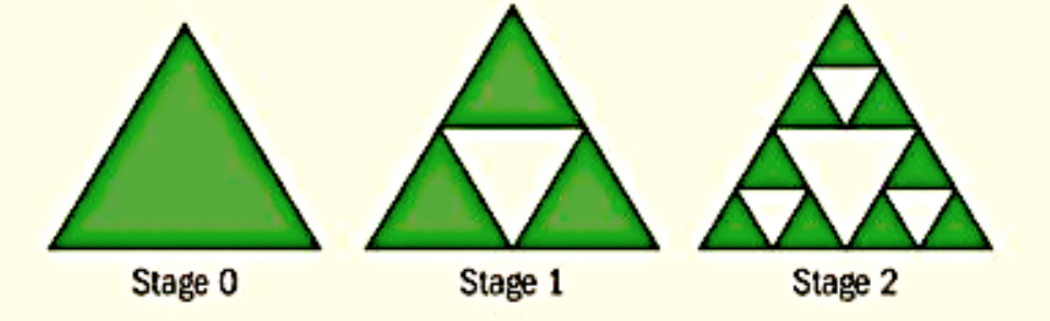
Well, anyway, for this task, we need to, first, find the next stage of Sierpinski’s triangle by observing the pattern between the first three stages then applying this pattern to get the next stage. Next, we had to fill out a table on the information about the number of green triangles, the length of one side of one green triangle and the area of each green triangle for stages 0 to 3, find the patterns of the first three rows of this table, what they have in common, find a formula to find the above info for triangles of stages 4, 5, 6, etc. and compare the numbers we obtained.

The topics involved are, again, geometry, specifically of triangles, perimeter and area of a triangle, infinity, geometric sequences and/or trends between sets of numbers.

We can see that the number of green triangles is a geometric series with the formula of 3^(stage no).

As for the length of one side of one green triangle, the formula is 1/2^(stage no), in other words it’s also a geometric sequence.

The area of each green triangle’s formula is 1/4^(stage no). Surprise, surprise, it’s also a geometric sequence.

All these three patters are geometric sequences; you find the next term by multiplying the pervious term with a fixed constant.

Therefore, if we we wanted to find the patterns for the 4th, 5th and 6th stages, it would be like the above table.

I could compare the sets of numbers ordained by lining up the sequences above one another and seeing the constants for each geometric sequence. We can then see the similarities in the numbers we’d get using the formulas we have and the similar ratio between same stage, different sequence numbers, which would all make up its own geometric sequence.

Sierpinski’s triangle is, again, infinite, as there will always be a space for a new triangle inside of the already existing triangles. As the size of the triangles decreases, the area of each triangle decreases, while, funnily enough, the total perimeter of the triangles increase suntil it approaches infinite. This happens because the area of the triangles decreases as the space for the triangles decreases while the quantity of the triangles increases. This results in an infinitely decreasing area and an infinitely increasing perimeter.

And so concludes the end of my triangle musings that lasted from morn to night as I followed in Koch’s and Sierpinski’s (triangle) steps.

If you’d like to explore more of the build of Sierpinski’s triangle, feel free to explore this link:

https://blogs.scientificamerican.com/roots-of-unity/a-few-of-my-favorite-spaces-the-sierpinski-triangle/

Reflection

From these investigations, I find I acquired better knowledge of geometric patterns and how shapes, triangles in particular, have a pattern with their perimeter and area. Triangles can also expand infinitely as snowflakes as exemplified by Koch’s snowflakes. As for skills I acquired, I found that I can assume sequences more quickly and find a pattern with triangles as well as think spatially better with these geometric investigations.

I can use these skills in my life to find a pattern in the happenings in my life and learn to manipulate the information I have to understand the context of something that is not necessarily mathematical better. This could be helpful in social situations where I have to watch out for social cues and can put a stop to any damaging patterns, such as snacking, I find in my life.

IB Learner Profile

IB learners are open-minded, knowledgable thinkers. IB learners are individuals who develop and use a good foundational understanding to explore many different subjects using critical and creative thinking to analyse the problem before them from many different points of view that would give them the chance to further their understanding.

With these exercises, I became more open-minded with the ways I can use and manipulate the information I have geometrically. I was also able to think more critically as I struggled to initially find the pattern between the sequences and numbers and, especially, find the perimeter and area of the triangles in investigation B. Lastly, I became more knowledgable of the geometry behind seemingly complex shapes such as snowflakes that really are just infinite triangles as well as the pattern existing in nature of these snowflakes and how sequences work.

Unforgettable Moments: me and math mutually tearing each other apart ver.

#igcsemath2020
#firstbatch TT

Sadly, I’m not one to take a lot of photos nor do I have too many memories to reminisce, however, I can show you this meme as a representation of how I felt as I finished writing my first math journal meme.

I had to write an journal and just being blown away with all the things we could do with our blog, though, granted, I’m still unable to achieve my ideal blog even with all these features due to many factors including my shortcomings and lack of understanding of wordpress. I won’t, however, rue the first time I published my e-journal and the euphoria of having my own place in the world wide web.

Bibliography

Interactivate: Sierpinski’s Triangle. (2019). Retrieved 20 November 2019, from http://www.shodor.org/interactivate/activities/SierpinskiTriangle/
Lamb, E. (2019). A Few of My Favorite Spaces: The Sierpinski Triangle. [online] Scientific American Blog Network. Available at: https://blogs.scientificamerican.com/roots-of-unity/a-few-of-my-favorite-spaces-the-sierpinski-triangle/ [Accessed 20 Nov. 2019].
athall, J., Harcet, J., Harrison, R., Heinrichs, L. and Torres-Skoumal, M. (2019). Education Bookshelf Mathematics Analysis and Approaches Higher Level. [online] Bookshelf.oxfordsecondary.co.uk. Available at: https://bookshelf.oxfordsecondary.co.uk/contents/428/index.html [Accessed 30 Oct. 2019].
Go Figure. (2019). Koch Snowflake. [online] Available at: http://gofiguremath.org/fractals/koch-snowflake/ [Accessed 20 Nov. 2019].
(2019). [Video]. Retrieved from https://www.deviantart.com/mezzaninex/art/Sierpinski-Triangle-Variation-53820973
(2019). [Video]. Retrieved from https://www.deviantart.com/mezzaninex/art/Sierpinski-Triangle-Variation-53820973

“The introduction of numbers as coordinates is an act of violence.”

Hermann Weyl, Philosophy of Mathematics and Natural Science

Part 1

Hermann Weyl must’ve struggled to comprehend that topic you have in your textbook about using matrices to transform a shape, because he doesn’t seem too pleased about matrix transformations, at least judging from the quote above.

While Hermann Weyl could’ve wailed all he wanted about his mathematical and philosophical woes, however, we 14-15-year-olds have an IGCSE to face that will definitely have at least one question about matrix transformations. So, how do we do it?

Matrices

A matrix is a rectangular array of numbers or other mathematical objects for which operations such as addition and multiplication are defined.

We can see the order of a matrix (row by column) from the above picture.

Operations

The operations we can do with a matrix at IGCSE level includes the following:
– Addition
– Subtraction
– Multiplication by Scalar
– Multiplying Matrices
– “Division”

Adding Matrices

As you can see, adding matrices is pretty simple. We simply add numbers in the same position together. In the above example, the sum of the numbers 4 and 1, both at the top, leftmost spot in their respective matrices, is the top, leftmost number in the new, resultant sum matrix.

Subtracting Matrices

The concept stays the same for subtracting matrices; simply subtract numbers in the same position together. For example, the difference between the numbers -1 and 3, both at the top, leftmost spot in their respective matrices, is -4, which is placed at the top, leftmost number in the new, resultant matrix.

Multiplication by Scalar

Multiplication by scalar is a little different. Here, the scalar (the constant, which is 2 in this case) by every number in the matrix to get the resultant matrix.

Multiplying Matrices

Multiplying matrices is where I believe Weyl’s brain began its road to hell, though it doesn’t have to be the same for you, reader.

First, there is a condition that needs to be fulfilled for multiplying between matrices to happen. The number of columns the first matrix must be the same as the number of rows of the second matrix; or (the matrices need to have the orders of AxB and BxC respectively in that order). This means that matrices like these:

which have the orders of 2×4 and 3×4 respectively, can’t be multiplied.

Now, we need to find the dot product of the rows and columns, which essentially mean this:

In this particular example, we need to do the dot product 4 times, till we get this:

This is a formula we can use, which is admittedly more complicated than the above method but you can use if it’s easier for you:

The placement of the dot products is from left to right from top to bottom, just like how we read.

Note that matrix multiplication is not commutative. In other words, the order of the matrices matter since AxB is not equal to BxA, unless…

one of the matrices is an identity matrix, which is:

– a square matrix (same number of columns as rows)
– all numbers are 0
– except for numbers that are part of the principal diagonal, which is a diagonal line from top, leftmost to bottom, rightmost.

This is an identity matrix:

Any matrix multiplied by the identity matrix will result in the same initial matrix.

“Division”

When I say divide, I don’t really mean divide, rather I mean multiplying with a matrix’s inverse. Like this:

Matrices can also have an inverse if they’re
– not singular
– a square matrix.

Singular matrices are matrices whose determinant is 0. The determinant of a matrix depends on its order. For IGCSE level, we only need to be able to find the determinant of matrices whose orders are 2×2 and 3×3, like such:

The formula for a matrix’s inverse is this:

For IGCSE level, we only need to know the inverse of a 2×2 matrix.

Transformations

Now, as you’ve probably guessed, matrices can represent coordinates. But how can these simple arrays of numbers possibly represent coordinates on a 2-D plane or even transform them?

Well, like this:

The top row represents the x-axis and the bottom row the y-axis.
Column 1 represents the coordinates of point D, column 2 the coordinates of point E and so on.

Coordinate matrices don’t necessarily have to form shapes. They may just be the matrix of a coordinate. Nonetheless, these matrices can still be transformed.

Transformations

There are 4 types of transformations:
– Rotation
– Translation
– Reflection
– Enlargement

Rotation
If an object is ‘rotated’, this means that it is turned a specific number of degrees around a centre point.

Translation
If an object is ‘translated’ this means that it is moved up, down, left or right of its original position on a grid. When translating an object, its shape size and direction remain the same.

Reflection
If an image is ‘reflected’, this means that it faces the opposite direction of the original object.

Enlargement
If you ‘enlarge’ or ‘resize’ an object, this means that you change its size but keep its original shape the same. In order to carry out enlargements, you need to know the scale factor of the object and the centre of enlargement.

Matrix Transformation

Now, there are ways to transform a coordinate matrix by multiplying it with other, specific matrices.

Here’s the list:

You may wonder why these specific matrices can transform coordinate matrices. Well, the best answer I can give you is that these matrices are all based on the identity matrix, just with some negatives and changing around in places. If you multiply one of these matrices with a coordinate matrix, I can guarantee you the resultant coordinate matrix will form a shape that is the original shape from the original coordinate matrix transformed.

Part 2

Uses of Matrices and Tranformations

Matrices are used in real life to render video game visuals since graphics software use matrices to process linear transformations to render images.

Matrices are also used by engineers in order to model physics systems and find the accurate result for complex calculations to allow machinery to work.

Transformations more specifically, on the other hand, are used in the mass production of glasses. After all, we need reflection to ensure the two sides of spectacles are symmetrical since even the smallest degree of imbalance can cause great discomfort to the wearer.

Part 3

IB Learners are knowledgable and reflective individuals. Through this e-journal, I was able to reflect on the ideas I absorbed during class and think on how I can apply them and solve problems with them. With this lesson, I increase my knowledge on maths and the limits of my math capabilities expands. I can show this by critically thinking and answering math problems with these new concepts in mind.

“I believe that we do not know anything for certain, but everything probably.” 

–Christiaan Huygens

Part 1

In so many things in life, it can’t be helped that we aren’t 100% sure of what will happen. So many are the unknown unknowns and the unknown knowns that at best, we can only say that something will happen … probably. Luckily, math, as our usual reliably torturous subject, does away with all the uncertainty and allows us to calculate the probability of a certain event happening.

Before we delve too deeply into probability, however, lets reflect on sets.

Sets

A set is a collection or group of distinct objects. Some examples of sets include:

A = {x : x is a positive odd number less than 10}

Then A = {1, 3, 5, 7, 9}

B is the set of days in a week.

Then B = {Monday, Tuesday, Wednesday, Thursday, Friday, Saturday, Sunday}

The objects in a set are known as elements of the set. For example, in the above examples I gave, 1, 3, 5, 7, 9 are all members of set A. This can be written in set notation as 3∈A (3 is a member of A).

Sets can also be empty of null, represented by the set notations ∅ and {}.

Sets can also be universal, wherein a set contains all possible elements. For example, a set of real numbers could be the universal set of a set of even numbers.

Sets can have subsets. This means that the members of the set and subset overlap as seen below.

You can see a more complete explanation for all the set notation symbols below.

These set notations and the sets themselves can then be show in the form of Venn diagrams.

Probability

Probability is a branch of mathematics that allows us to analyze random experiments. In other words, if we’re given data on the number of students wearing glasses, not wearing glasses, are female and are male, we can reasonably get the probability of the likeliness of getting a male student who wears glasses if we picked a random student from the class.

In probability, a 0 means that an event won’t happen – it is impossible – and a 1 means the opposite – it will definitely happen. All probabilities lie between these two numbers, in fraction or decimal.

Below are some probability formulas.

Mutually exclusive events mean that the two events are, in reference to a venn diagram, disjoint or have no intersection. Non-mutual events or combined events are events where the two events do have an intersection (hence why in the above formula the intersection of A and B was subtracted; to prevent overlap of members).

Conditional probability is the likeliness of one event occurring with some relationship to one or more other events.

For example, we have a deck of cards (typical), and draw two cards without returning any. We want to calculate the probability of drawing a Jack the first draw and drawing another Jack the next draw.

For the first draw, the probability of drawing a Jack is 4/52.

P(A)=4/52

Since we don’t return the cards, for the second draw, the likeliness of drawing a Jack becomes 3/51.

In set notation, this can be written as:

P(A and B) = P(A) x P(B|A) = (4/52) x (3/51) = 12/2652 = 1/221

We can depict probability by using tree diagrams, like in the below example of a tree diagram for the probabilities of a coin flip.

Tree diagrams allow us to easily see the probability of singular events (the numbers on the branches), but aren’t convenient for questions with many outcomes (draws/tosses).

Sometimes you may also be asked for the relative frequency of an event. Do not fear, this just means the question is asking you for the probability of that event in percentage of decimal form.

Part 2

Uses of Sets and Probability

Since sets are just a collection or group of distinct objects, the real life uses of sets is more to just describing of what is in a certain group.

For example, a spotify playlist titled ‘Women of K-Pop’ would include songs made by Korean female soloists or groups in the pop genre and would not include blues songs.

Another example is that a school bag has different pockets for different objects. The biggest, middle division would be for textbooks, notebooks and any other bulkier objects while the front pocket would be for thinner, less essential objects like earphones.

Probability plays a large role in analysing insurance policies to decide which insurance most suits your needs. If your city is rampant with crimes and the local government publishes a study where, in your city, every 1 in 3 men can expect to experience an attempted assault on themselves once every 3 months, you would purchase an insurance that caters to this need. In other words, probability can help us make decisions.

While it is unfortunate and mildly depressing to know that life is almost entirely out of our control, calculating simpler probabilities can help us get a better grasp of what happens around us (and maybe win us some card games). Either way, enjoy life and know that one definite thing you can count on is life being unpredictable … probably.

"Facts are stubborn things, but statistics are pliable." -Mark Twain.

No matter what grade you become or how many exercise books you’ve finished, all math students will return to statistics, the science of collecting, analysing, presenting and interpreting data. Here, I’ll be reflecting on a statistics question mainly concerned about cumulative frequency, the cumulative frequency graph and measures of central tendency by way of doing and explaining how I solve an IGCSE question, specifically from the May/June Session of 2005 Paper 4 Question 7 and give a few real-life applications of statistics.

IGCSE Example Question

A common statistics question in the IGCSE is like the following:

As we can see, the question gives one variable, the speeds of 150 cars in v kilometers/hour and the cumulative frequency in a graph.

For (a)i), to find the median speed using the graph given, or the 50th percentile, we simply have to use the 1/2(n) or 1/2(n+1) formula (because 50/100(n) can be simplified to 1/2(n). Since 150 is already an even number, let’s save ourselves the trouble of a decimal number and just use 1/2(n).

So, 1/2(150)=75. 75 here doesn’t mean that the median speed is 65, but rather the place of the median speed is 75th in the cumulative frequency. So, we look at the y-axis and find the 75th place, which is roughly 46.5 km/h.

Next, for (a)ii), we need to consult the formula to find the interquartile range. IQR=Upper quartile – Lower quartile. The upper quartile is the 75th percentile of the data and the lower quartile is the 25th percentile. Therefore, we can use the formula above once again, though with a little tweaking. Since this time we’re finding the 75th and 25th percentile, we should put in 3/4(n) and 1/4(n) respectively (simplifications of 75/100 and 25/100 respectively).

Therefore, the place of the 75th percentile is 112.5th and the place of the 25th percentile is 37.5th. When we get places of decimal numbers like these, we have to take values of the place before it and the place after it and divide the sum by two. For example, for the 75th percentile, 112.5th place, we have to take the (112th + 113th)/2. This would be (51.5 + 52)/2=51.75. So the UQ is 51.75

As for the LQ, it would be (37th+38th)/2, which is (42+42.5)/2=42.25. So the LQ is 42.25

We can now insert these values into the IQR equation, which becomes IQR=51.75-42.25=9.5.

Finally, for (a)iii), the questions is asking for the number of cars that travel with speeds more than 50 km/h. This means that we must subtract the total number of cars with those that have speeds of and below 50 km/h since the question is king for speeds of more than 50 km/h, not less than (if it did it would’ve been just fine to find the cumulative frequency of cars through the graph by looking at the x-axis’s 50 and seeing the corresponding y value for that).

So, we know the total number of cars is 150. The number of cars that go below 50 km/h we need to find using the graph. It’s 112. So, we just have to do 150-102=48.

These are the next subquestions. For (b)i), we need to find the cumulative, not cumulative frequency, of the number of cars in each of the classes given. This can be done by, once again, looking at the graph. There are 134 cars driving at a speed of 55km/h while there are 102 that drive at a speed of less than 50 km/h. Therefore to find n, we do 134-102=32.

For (b)ii), to find the mean speed of the cars, we must find the midpoint of the classes in the table. Since this is a question with large data, not single data like 1 4 66 91, then we don’t need to mind the sign. We just add the minimum and maximum value of each class and divide it by 2. So for 30<v<=35, it’s (30+35)/2, which is 32.5. We repeat this process for all the other classes.

Speed (v km/h)	30<v<=35	35<v<=40	40<v<=45	45<v<=50	50<v<=55	55<v<=60
Frequency	10	17	33	42	n=32	16
Midpoint	32.5	37.5	42.5	47.5	52.5	57.5

Source: Made by me

We then get the table above. Then, we multiply all the frequencies with its class’ corresponding midpoint, add all the values up and divide them by the total number of cars.

So it’s (32.5×10 + 37.5×17 + 42.5×33 + 47.5×42 + 52.5×32 + 57.5×16)/150, which is 6960/150=46.4.

For (c), we need to make a histogram with the values given in the table. However, for this, we can’t just use the frequency as the y-axis. For histograms, we need to use frequency density, which is basically the frequency/class width (maximum value of class – minimum value). So if it’s for class 30<v<=40, we’d have to do 27/(40-30)=2.7. Again, no need to mind the signs for class width.

Speed (v km/h)	30<v<=40	40<v<=55	55<v<=60
Frequency	27	107	16
Class Width	10	15	5
Frequency Density	2.7	~7.13	3.2

Source: Made by me

The resulting class widths and frequency densities will be like the above. Finally, we make the histogram making 2 cm for 5 units on the speed axis (x-axis) and 1 cm to represent 1 unit on the frequency density axis (y-axis); following the instructions of the question. The resulting histogram should be like this:

Real-Life Applications of Statistics

How do you think weathermen tell you the weather forecast. Do they pick out a random slip of paper with a random weather Hunger-Games style? Do they open up a fortune cookie from the nearby Chinese Take-Out place? Did God tell them? Well, no. The weather forecast is partly based on computer models that use statistics. That’s right, lots and lots of data is compared to previous weather data to predict if there’ll be a flood or not tomorrow.

Another application of statistics in real life is in medical studies, or more technically, medical statistics. Medical papers use a range of statistics to prove their point. If there weren’t reliable numbers, we could well be consuming poisonous silver nitrate instead of proper drugs that can cure us of illness. Indeed, if doctors didn’t learn how to make histograms properly, the world mortality rate might be a lot, lot lower than it is now.

As you’ve read for yourself, statistics are a very incredible thing, though still a bit of an irritating and time-consuming question to do in the IGCSE. Thank you for taking the time to read this journal entry of mine and I hope you close this page with a better understanding of how to approach a statistics question when, inevitably, IGCSE looms around your corner.

-T. Isabella